
The language behind raster analysis
Map algebra is a conceptual language designed specifically for cell-based geographic information systems. It provides the theoretical foundation for cartographic modeling, that is, using maps not just to display data, but to analyze and derive new spatial information.
The idea of map algebra comes from work originally presented by Joe Berry and C. Dana Tomlin, who recognized that raster maps could be treated as mathematical objects while still preserving their geographic meaning.
At its core, map algebra:
- Treats a raster map as a grid of values tied to real-world locations
- Applies operators and functions to entire maps, not individual numbers
- Allows users to express logic, conditions, and mathematical relationships in a structured way
This is what makes map algebra different from matrix algebra. While matrix algebra operates on abstract numeric arrays, map algebra operates on spatially referenced grids, ensuring that every calculation respects geography (location, extent, resolution).
In practical terms, map algebra provides:
- A clear vocabulary for expressing spatial logic (e.g., comparisons, thresholds, combinations)
- A mathematical backbone for raster operations
- A framework that naturally leads to local, focal, zonal, and global functions, each defined by how much spatial context is used in a calculation
GIS Functions and Operators
In raster-based GIS, functions and operators describe how values in a raster are processed to create new information. The key difference between these functions is how much surrounding information each cell “looks at” when a calculation is performed. Some functions operate on a single cell at a time, changing values based only on what is already in that location. Others expand the context to include neighboring cells, groups of cells that belong to the same zone, or even the entire raster dataset. In addition, some functions are designed for specific analytical purposes, such as modeling water flow or terrain characteristics. Together, these categories provide a structured way to understand how raster data can be transformed, analyzed, and modeled in GIS.
In the following sections, we will explore each of these operator types – local, focal, zonal, and global – in more detail, focusing on how they work, what spatial context they use, and when each is most useful in GIS analysis.
Local Operators (Local Functions)
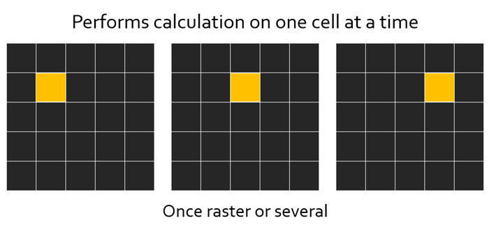
Local operators are the simplest and most intuitive type of raster operation. They work by applying a calculation to one cell at a time, then moving on to the next cell, until the entire raster has been processed. The key idea is that each cell is treated independently – the result for a given cell depends only on the value at that same location, not on neighboring cells or broader spatial patterns.
To perform a local operation, the function only needs:
- The value of a single cell from one raster, or
- The values of corresponding cells from multiple rasters, or
- A cell value compared against a constant or threshold
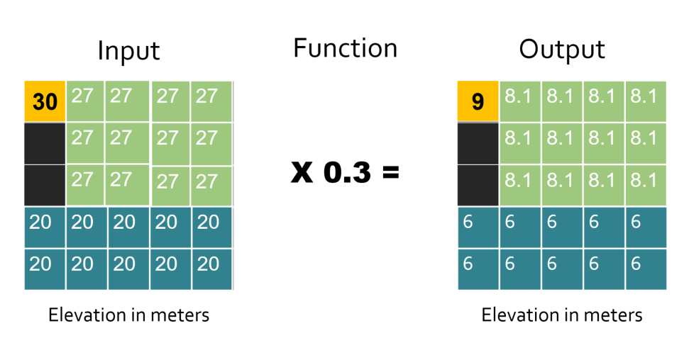
Because of this, local operators are often used for reclassification, unit conversion, conditional logic, and raster arithmetic. They are especially powerful for combining multiple raster layers, such as elevation, land cover, or climate variables, where each output cell represents a direct mathematical or logical result of the inputs at that exact location.
In map algebra terms, local operators are where raster analysis usually begins—they establish the basic cell-by-cell transformations that more complex spatial analyses build upon. See example below:
Some commonly used local tools in ArcGIS Pro include:
- Raster Calculator – Performs mathematical and logical expressions on raster cells
- Reclassify – Assigns new values to cells based on value ranges or categories
- Con (Conditional) – Applies if/then logic to raster cells
- Cell Statistics – Computes statistics for each cell across multiple rasters
Cell Statistics with solar potential layers
A clear way to demonstrate a local operator is by using Cell Statistics with a stack of monthly solar potential rasters. In this case, each raster represents solar potential for a different month of the year, but all rasters share the same extent and cell alignment.
Using the Cell Statistics tool, you can calculate:
- Mean solar potential for each cell across all months (average annual potential)
- Minimum solar potential for each cell (lowest monthly value)
- Maximum solar potential for each cell (highest monthly value)
For each output cell, the tool looks only at the values from the same cell location across all input rasters. No neighboring cells are considered, which makes this a classic local operation. The result is a new raster where each cell summarizes how solar potential varies over time at that specific location.
Focal Operators (Focal Functions)
Focal operators, also known as neighborhood operations or moving window operators, calculate a new value for each cell based not only on that cell itself, but also on the values of the surrounding cells in its neighborhood. Like local operations, focal operations still process the raster one cell at a time—but the calculation for each target cell depends on a defined group of nearby cells.
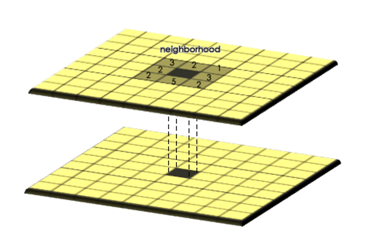
You can think of a focal operation as placing a window over the raster, centered on a specific cell. All the cells inside that window are used to compute a value, which is then assigned to the center (or focal) cell. The window then shifts to the next cell, and the process repeats until the entire raster has been processed
Neighborhoods can vary in both size and shape, depending on the phenomenon being modeled. Common neighborhood geometries include:
- Rectangles or squares (e.g., 3×3, 5×5)
- Circles
- Annuli (rings, where the center cell is excluded)
- Wedges or directional neighborhoods
These shapes are important because they allow focal operators to better represent real-world spatial processes. For example, a wedge-shaped neighborhood can be useful for modeling directional phenomena, such as ocean currents or prevailing winds.
A wide range of statistical and arithmetic functions can be applied within a neighborhood, including mean, sum, minimum, maximum, variety (number of unique values), and more. To illustrate how this works conceptually, imagine calculating variety. For each window position, the tool counts how many different values exist within the neighborhood. If there are four unique values, the output cell receives a value of four. The window then moves to the next cell and repeats the calculation. This type of operation is often used to measure spatial heterogeneity or variation. Most focal tools also allow you to control how NoData values are handled, such as ignoring them or filling gaps.
Some commonly used focal tools in ArcGIS Pro include:
- Focal Statistics – Calculates statistics (mean, sum, min, max, variety, etc.) within a moving window
- Neighborhood Statistics – Advanced neighborhood-based summaries
- Filter – Smooths or sharpens rasters using neighborhood kernels
Consider a raster dataset representing solar radiation or solar power potential, where each cell stores the estimated solar energy received at that location. A local value alone tells us how much sunlight a single point receives, but in many real-world applications—such as planning solar installations—we care about conditions in the surrounding area, not just one pixel.
Using a focal operator, we can calculate the mean solar potential within a neighborhood (for example, a 5×5 or circular window). This produces a raster where each cell represents the average solar potential of nearby locations, not just the cell itself.
This approach is useful because:
- Solar panels are installed over areas, not single cells
- Small shadows, noise, or modeling artifacts are smoothed out
- It highlights consistently sunny regions, rather than isolated high-value pixels
For example, applying Focal Statistics (Mean) to a solar potential raster helps identify broad zones with stable, high solar energy—ideal candidates for solar farms.
Focal operators can also be used to measure spatial variability in solar potential. By applying a focal operation such as Range or Standard Deviation, students can see how much solar energy varies within a neighborhood.
- Low variability areas suggest uniform exposure (flat, unshaded terrain)
- High variability areas may indicate shading effects from terrain, buildings, or vegetation
This is especially helpful in urban or mountainous environments, where solar potential can change rapidly over short distances.
Another video to see an example of focal tools, in this particular case, the video addresses Raster Block and Focal Statistics:
Zonal Operators (Zonal Functions)
Zonal operators analyze raster values based on predefined zones. Instead of focusing on individual cells (local) or moving neighborhoods (focal), zonal operations work one zone at a time. A zone is a group of cells that share the same value in a separate zone dataset, which can be either a raster or a vector layer (for example, land parcels, watersheds, administrative boundaries, or land cover classes).
To perform a zonal operation, two datasets are required:
- A zone layer, which defines where calculations will occur
- A value raster, which contains the data being summarized
The zone layer controls the analysis. For each zone, the tool gathers all raster cells that fall within that zone and applies a statistic—such as mean, sum, minimum, maximum, or majority. The result is one value per zone, not per cell neighborhood.
For example, if a raster contains three zones and you calculate the mean, the zonal operator:
- Takes all raster values in Zone 1 and computes a single mean
- Repeats the process independently for Zone 2 and Zone 3
In the output raster, every cell within the same zone receives the same value, reflecting the statistic calculated for that zone. This is a key difference from local and focal operators, where output values can vary from cell to cell even within the same area.
Zonal operations are especially useful when the question is:
“What is the overall value of this variable within each defined region?”
Imagine you have a solar potential raster and a polygon layer representing counties or census tracts. Using a zonal operator, you can calculate:
- The mean solar potential per county
- The maximum solar potential within each tract
- The majority solar class for each region
This allows students to move from a continuous raster surface to region-based summaries, which is how many real-world planning and policy decisions are made.
Instead of asking “Which cells are sunny?”, zonal analysis asks:
“Which regions, as a whole, have the highest solar potential?”
Some widely used zonal tools in ArcGIS Pro include:
These tools are commonly applied in environmental analysis, land-use planning, resource management, and renewable energy modeling—making zonal operators a critical bridge between raster analysis and decision-making at meaningful geographic scales.
Some widely used zonal tools in ArcGIS Pro include:
- Zonal Statistics – Calculates statistics (mean, sum, min, max, majority, etc.) for raster values within each zone
- Zonal Statistics as Table – Outputs the same statistics in tabular form
- Tabulate Area – Computes the area of raster classes within each zone
- Zonal Geometry / Zonal Geometry as Table – Computes geometric properties of zones
These tools are commonly applied in environmental analysis, land-use planning, resource management, and renewable energy modeling—making zonal operators a critical bridge between raster analysis and decision-making at meaningful geographic scales.
Global Operators (Global Functions)
Global raster operators take into consideration every single cell in a raster dataset in order to calculate a value for any one cell. While this may sound redundant at first, it is important to emphasize this point because it highlights how global operators differ from all other raster operation.
In global operations, the calculation for a single output cell may depend on information from the entire raster extent. In conceptual diagrams, this is often shown by highlighting all cells (for example, in red) to indicate that every cell contributes to the result, even if the final value is assigned to just one location.
Global (or per-raster) functions compute an output raster where the value at each cell is potentially a function of all cells combined from one or more input raster datasets. Because they rely on complete spatial context, global operations are usually computationally expensive and may take longer to process, especially for large datasets.
Global operators are most commonly used to model spatial connectivity, movement, or influence across an entire landscape, rather than localized or regional patterns.
Two common global raster operations include some of the proximity analysis tools:
- Euclidean Distance: Calculates the straight-line distance from each cell to the nearest source cell (such as roads, rivers, or buildings). Example application: Identifying areas farthest from infrastructure or services.
- Weighted Distance (Cost Distance): Calculates distance while accounting for resistance or cost across the landscape (such as slope, land cover, or barriers). Example application: Modeling least-cost paths for wildlife movement or energy transmission routes.
Another important class of global raster operations is interpolation analysis.
Interpolation estimates values at unsampled locations by using all known input points across the study area. Although the output is a raster where each cell receives its own value, the calculation for each cell depends on the overall spatial distribution of input data, not just nearby cells. This makes interpolation a global operation.
Common interpolation methods include:
- Inverse Distance Weighting (IDW) is a spatial interpolation method used to estimate values at locations where no data was collected. It works on the idea that places closer to each other are more similar than those farther apart, so nearby measured points have more influence on the estimated value than distant ones. IDW is simple to use and works best when data points are evenly distributed, but it does not measure uncertainty or prediction error.
- Spline is a spatial method used to estimate values at locations where no data was collected by creating a smooth surface that passes through the known data points. It assumes that changes between points happen gradually, so the surface bends gently to fit the input values. Spline works well for smoothly varying data, such as elevation, but it can create unrealistic values if the data changes sharply or contains outliers.
- Kriging is a spatial interpolation method used to estimate values at locations where no data was collected by analyzing how values change with distance and direction. It assumes that nearby locations are more similar than distant ones and uses this spatial pattern to make predictions. Kriging not only estimates values but also provides a measure of uncertainty, making it a more advanced and statistically based method than other interpolation techniques.
Check the following link to explore the differences between the interpolation methods: Comparing Interpolation methods (ESRI).
Example application: Suppose you have point measurements of solar radiation, temperature, or wind speed collected at weather stations. Interpolation uses those point values to create a continuous surface that estimates conditions everywhere across the landscape. Each cell’s value reflects how it relates to all sampled locations, weighted by distance, spatial trends, or statistical relationships.
Interpolation is widely used in:
- Climate and environmental modeling
- Renewable energy assessment (solar, wind)
- Air quality and pollution studies
Even though interpolation produces values cell by cell, each value is influenced by the entire dataset of observations. That reliance on global context—rather than a fixed neighborhood or zone—is what places interpolation firmly in the category of global raster operators.
Other global operation tools are:
- Flow Direction is a function that analyzes a digital elevation model to determine how water moves across the entire surface. Although a direction value is assigned to each cell, the analysis depends on understanding how all cells are connected across the landscape, making it a global operation.
- Viewshed is a spatial analysis tool used to determine which areas of a landscape are visible from one or more observation points. It analyzes the terrain surface and checks line-of-sight between the observer and surrounding locations, taking into account elevation and obstacles. The result shows areas that are visible and not visible, and it is commonly used in applications such as site planning, landscape analysis, and visibility studies.
Why Raster Operations Matter
Raster-based GIS offers a wide and powerful set of cell-based modeling functions developed to support many different analytical applications. While we often classify raster operations as local, focal, zonal, or global, it is important to recognize that these categories are not rigid. Many tools can belong to more than one conceptual group depending on how they are used. For example, slope is commonly associated with surface analysis, yet it is fundamentally a focal operation because it relies on a cell’s neighborhood.
Because of this flexibility, raster operations play a critical role in a wide range of spatial assessments, including land evaluation, environmental modeling, hazard analysis, and renewable energy planning. In a typical land evaluation workflow, GIS supports each major step of the process:
- Initial consultations to define objectives, assumptions, and data needs
- Land use analysis to describe potential uses and their requirements
- Land characterization to define mapping units and derive relevant land qualities
- Comparative assessment to evaluate how different land uses perform across land types
- Economic and social analysis to assess feasibility and impacts
- Land suitability classification to assign qualitative or quantitative rankings
- Presentation of results, often through an iterative and exploratory process
GIS significantly enhances these workflows by allowing analysts to integrate data, apply consistent spatial logic, and visualize results clearly. However, effective analysis depends not only on software capabilities, but also on careful planning, realistic expectations about time and resources, and—most importantly—a clear understanding of the available tools and methods.
A solid grasp of local, focal, zonal, and global raster operations provides the foundation needed to design meaningful analyses, interpret results correctly, and apply GIS responsibly in real-world decision-making.
Suggested sources for further reading
- Tomlin, C. D. (1990). Geographic Information Systems and Cartographic Modeling.
- Berry, J. K. (1993). Beyond Mapping: Concepts, Algorithms, and Issues in GIS.
- ESRI Documentation: Raster Analysis and Map Algebra
- Burrough, P. A., & McDonnell, R. A. (1998). Principles of Geographical Information Systems.